Chaos Game - Creating Fractals using Simulation
Fractals are objects that are infinitely rough, the idea is that no matter how close one zoom in, one can see some detail of the pattern. Interestingly, the fractals that we generate will be self similar, meaning that if we zoom into one part of such pattern, you should be able to see the entirety of the pattern again.
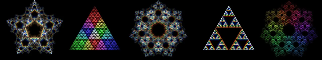
In this guide, we are going to talk about how to generate some of these fractals using for loops and random package in python.
Generate a Sierpinski Triangle
First, let us start with an equilateral triangle, as shown below.
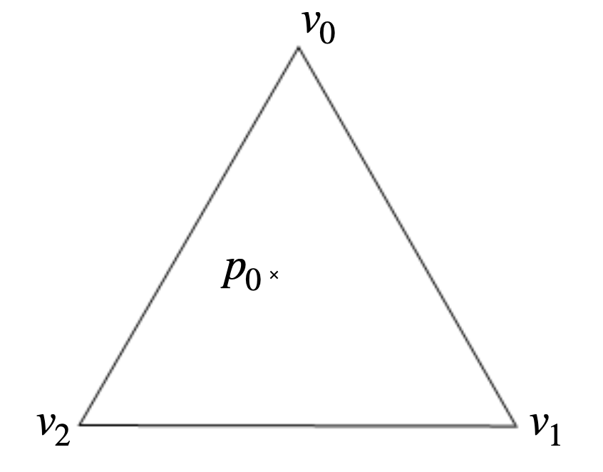
We denote each of the vertices as $v_0$, $v_1$ and $v_2$.
In python, we can define the points using a 2-dimensional cartesian coordinate system:
Each time, pick a vertices $v_r$ of the triangle with equal probability. $r = 0, 1, 2$
Start from an initial point $p_t$, we set the next iteration of the point using the following formula:
$$ p_{t+1} = \frac{p_t + v_r}{2}$$.
Here is an example of such iteration:
Say that the random vertices we have chosen is $v_1$, then we have the following $p_{t+1}$
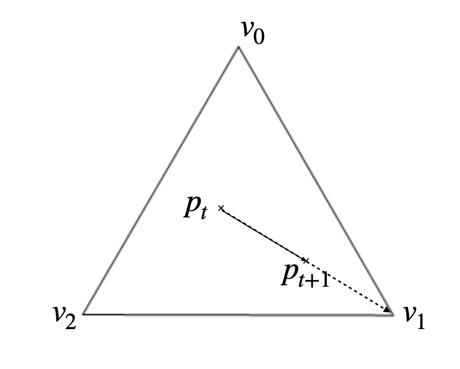
We can use the same iteration rule to update our current point.
Let us evolve the point from now on and see how it looks like. You can use the for loop to simulate this process in python:
from numpy.random import randint, choice
xss, yss, clrs = [], [], []
crt_x, crt_y = trig_xs[0], trig_ys[0]

for i in range(1,80000):
    randidx = randint(0,len(trig_xs))
    # randidx = choice(3,p=[0.49,0.02,0.49])
    vet_x, vet_y = trig_xs[randidx], trig_ys[randidx]
    crt_x, crt_y = (vet_x + crt_x)/2, (vet_y + crt_y)/2

    clrs.append(randidx)
    xss.append(crt_x)
    yss.append(crt_y)
Inside each for loop we are essentially repeating the above process over and over again.
Here randidx is a random number from the list [0,1,2]. The vet_x, vet_y is the x,y coordinate of the chosen vertices. The crt_x, crt_y stores the corrdinate of $p_t$. clrs stores which vertices has been chosen.
We iterate the above process for 80000 steps and we store the coordinate in the xss, yss.
After running the simulation, we can look at the result of our simulation using a scatter plot:
One should be able to see something like the following:
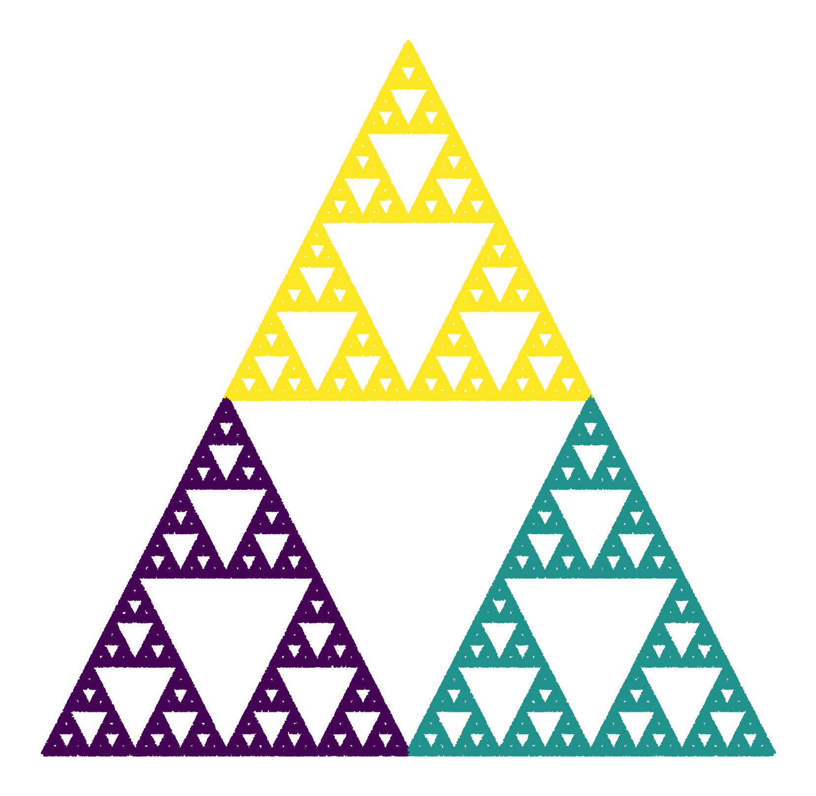
How amazing is that! Even though the process is completely random. The points neatly avoids all the center triangular reigon inside of a smaller triangle.
Here, I made an animation script so that you can see how the points come into being.
Run the following code in the notebook and you will see how each point contribute to making the shape:
from matplotlib.animation import FuncAnimation

plt.rcParams["animation.html"] = "jshtml" ## The format to output the animation
plt.rcParams['figure.dpi'] = 150 ## The resolution of the animation
plt.ioff()
fig, ax = plt.subplots(figsize=(7,7))

def grw_func(t): # Function dictating how the animation time frame grow
    if t < 70:
        return t
    elif t < 130:
        return 30*(t-70) + 70
    else:
        return 30*pow(t-130,3)+30*(t-70) + 70

def animate(t): # Function for static animation of the chaos game
    plt.cla()
    until_num = grw_func(t)
    ax.scatter(x=xss[:until_num],y=yss[:until_num],c=clrs[:until_num],marker='+') ## Plot the points up to until_num as a "x"
    ax.set_title('Step Number {}'.format(until_num))
    ax.set_xlim(-1,1)
    ax.set_ylim(-0.07,1.73)

FuncAnimation(fig, animate, frames=140)
This is truely amazing, a fun exercise would be to prove why the above procedure generate a fractal.
(For a hint, you could consider the induction problem. First, think about why there are no points in the middle triangle.
Then use mathematical induction to prove that there will never be any points in the middle triangle for all the smaller triangles.)
Restricted Square
Why stop at triangle, what if we consider a square.
Sadly, if we use the previous technique and always march half way for a random selected square vertices, the square will always fill up.
Luckily, there are some ways we can get around it.
We can ask the random points to follow some restrictions when marching towards the vertices.
First, we define the coordinate of the vertices:
Then we select a vertex as initial point $p_t$. Each time $t$, we select a random vertix $v_r^{t}$ of the square.
Then we update the point $p_t$ the same way as $$ p_{t+1} = \frac{p_t + v_r^{t}}{2} $$.
However this time, we choose $v_r^t$ such that it cannot be diagonal with $v_r^{t-1}$. In another words, $d(v_r^t, v_r^{t-1}) \neq \sqrt{2} $.
We can implement as following:
xss, yss, clrs = [], [], []
crt_x, crt_y = sq_xs[0], sq_ys[0]

last_idx, this_idx = 0, 0
for i in range(1,80000):
    # randidx = choice(3,p=[0.49,0.02,0.49])
    this_idx = randint(0,len(sq_xs))

    while np.abs(this_idx - last_idx) == 2:
        # print(this_idx)
        this_idx = randint(0,len(sq_xs))

    vet_x, vet_y = sq_xs[this_idx], sq_ys[this_idx]
    crt_x, crt_y = (vet_x + crt_x)/2, (vet_y + crt_y)/2
    last_idx = this_idx
    clrs.append(this_idx)
    xss.append(crt_x)
    yss.append(crt_y)
Here, we used the trick that this_idx and last_idx cannot be distance 2 from each other.
If we plot the result:
plt.figure(figsize=(14,14))
plt.scatter(xss, yss, c=clrs, marker='+')
plt.axis('off')
plt.show()
The result should be something like this:
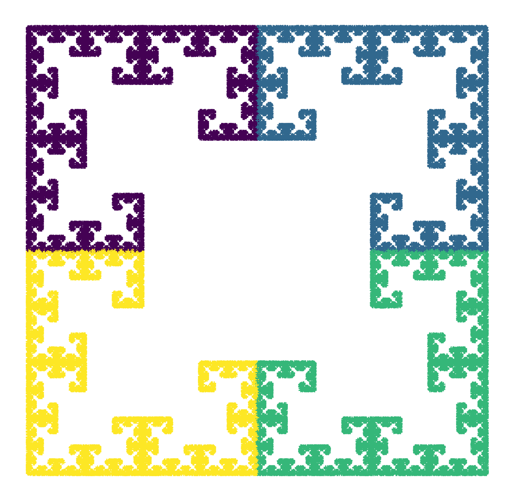
Note here, if we try different restriction rules, we can get entirely different fractal shapes! You can explore this by modifying the code above!
Other Generalizations
There are tones of beautiful and interesting chaos game to play around with, one of them is called barnsley fern.
It is a very intricate pattern of a fern leaf, but it is constructed by randomly selected one of the four linear transformations.
Here is part of the code which construct these linear transformations:
def generate_lineartransformation(a1,b1,c1,a2,b2,c2):
    def theF(x, y):
        # print(c2)
        return a1*x+b1*y+c1, a2*x+b2*y+c2
    return theF

f1 = generate_lineartransformation(.0,.0,.0,.0,0.16,.0)
f2 = generate_lineartransformation(.85,.04,.0,-.04,.85,1.6)
f3 = generate_lineartransformation(.20,-.26,.0,.23,.22,1.6)
f4 = generate_lineartransformation(-.15,.28,.0,.26,.24,.44)

f_idices = [0,1,2,3]
flst = [f1,f2,f3,f4]
prob = [.01,.85,.07,.07]
Using the similar idea and the code provided you can create intricate visualization such as below.

Additional resources
Here are some additional resources that you may find interesting: