Starting Your Own Data Science Project
Starting a data science project of your own can be an intimidating task. In this guide, we will help give you a head start on building your own project. We'll walk through: how to find a dataset, ways to start analyzing it, and some steps to spark ideas for you to explore!
Collecting Your Data
First, we need to find a dataset to perform our analysis on. It's best to find a dataset about a topic you are passionate about. As well, having prior knowledge about the data you're analyzing will help you understand the context behind certain columns which inform your analysis. Kaggle.com is a great resource to find a dataset on just about anything. If you are interested in sports for example, you can find more specific datasets at websites such as sports-reference.com.
For this example, we'll use a dataset of songs from our favorite artist at DISCOVERY; Taylor Swift!
The dataset we'll be using can be found on Kaggle, and contains information about every Taylor Swift song. Kaggle datasets also contain information about what the columns in the dataset represent.
Our columns in this dataset are Name (song name), Album, release_date, length, popularity, danceability, acousticness, energy, instrumentalness, liveness, loudness, speechiness, valence, and tempo. This may seem like a lot of information, so we'll take it slow and analyze a few of the variables at a time. Our first step will be to load the DataFrame, and become familiar with it so we can perform our analysis.
df = pd.read_csv('spotify_taylorswift.csv')
df.head(5)| name | album | artist | release_date | length | popularity | danceability | acousticness | energy | instrumentalness | liveness | loudness | speechiness | valence | tempo | |
|---|---|---|---|---|---|---|---|---|---|---|---|---|---|---|---|
| 0 | Tim McGraw | Taylor Swift | Taylor Swift | 2006-10-24 | 232106 | 49 | 0.580 | 0.575 | 0.491 | 0.0 | 0.1210 | -6.462 | 0.0251 | 0.425 | 76.009 |
| 1 | Picture To Burn | Taylor Swift | Taylor Swift | 2006-10-24 | 173066 | 54 | 0.658 | 0.173 | 0.877 | 0.0 | 0.0962 | -2.098 | 0.0323 | 0.821 | 105.586 |
| 2 | Teardrops On My Guitar - Radio Single Remix | Taylor Swift | Taylor Swift | 2006-10-24 | 203040 | 59 | 0.621 | 0.288 | 0.417 | 0.0 | 0.1190 | -6.941 | 0.0231 | 0.289 | 99.953 |
| 3 | A Place in this World | Taylor Swift | Taylor Swift | 2006-10-24 | 199200 | 49 | 0.576 | 0.051 | 0.777 | 0.0 | 0.3200 | -2.881 | 0.0324 | 0.428 | 115.028 |
| 4 | Cold As You | Taylor Swift | Taylor Swift | 2006-10-24 | 239013 | 50 | 0.418 | 0.217 | 0.482 | 0.0 | 0.1230 | -5.769 | 0.0266 | 0.261 | 175.558 |
Exploring the Dataset
This dataset has 171 rows, and by using the pandas function df.dtypes(), we can see the data types of each column. Variables such as album name, artist name etc. are coded as objects, while audio information is numerical and is represented by integer or float values.
When working with datasets from the internet, the data might not always be perfectly formatted. There could be missing values, or data may have been entered incorrectly due to human error. Due to the imperfect nature of some datasets, it is important to understand what each column is supposed to be representing. This dataset seems to have the data types we'd expect for each column, so we can proceed.
If your dataset has null or missing values, or an incorrect data type (such as an object where an int or float value should be), you can look at our guide on handling missing data here to see how to correct it.
print('Dataframe Length: ' + str(len(df)))
print(df.dtypes)
Dataframe length: 171
name object
album object
artist object
release_date object
length int64
popularity int64
danceability float64
acousticness float64
energy float64
instrumentalness float64
liveness float64
loudness float64
speechiness float64
valence float64
tempo float64
dtype: object
Descriptive Analysis
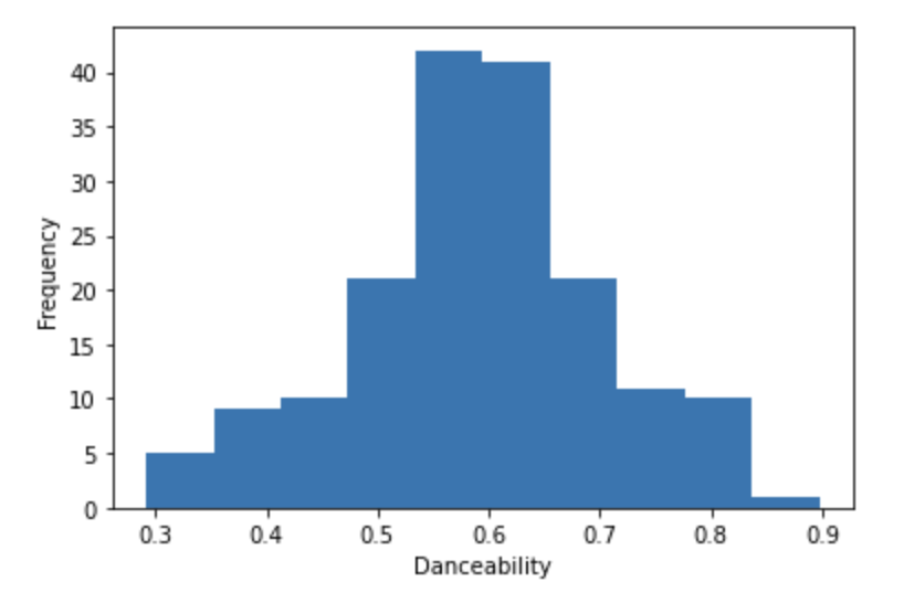
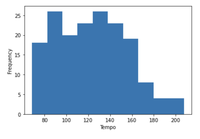
Our next step will be to explore the dataset in order to find relationships that interest us. It can be helpful to plot out variables of interest, and as you can see below, we plotted histograms for the popularity, danceability, and tempo variables.
Popularity is given as an integer ranging from 0-100, danceability is a metric ranging from 0-1 measuring how suitable a song is for dancing, and tempo measures beats per minute. Note that danceability appears to be normally distributed.
We can use functions such as df.describe() or df.corr() to see if there are any strong numerical relationships or variables with especially high/low values that we may want to inspect further.
df.describe()| index | length | popularity | danceability | acousticness | energy | instrumentalness | liveness | loudness | speechiness | valence | tempo |
|---|---|---|---|---|---|---|---|---|---|---|---|
| count | 171.0 | 171.0 | 171.0 | 171.0 | 171.0 | 171.0 | 171.0 | 171.0 | 171.0 | 171.0 | 171.0 |
| mean | 236663.52 | 61.228 | 0.589 | 0.322 | 0.586 | 0.002 | 0.146 | -7.322 | 0.066 | 0.423 | 124.141 |
| std | 40456.72 | 11.905 | 0.115 | 0.334 | 0.19 | 0.019 | 0.09 | 2.879 | 0.106 | 0.193 | 31.484 |
| min | 107133.0 | 0.0 | 0.292 | 0.0 | 0.118 | 0.0 | 0.034 | -17.932 | 0.023 | 0.05 | 68.534 |
| 25% | 211833.0 | 58.0 | 0.527 | 0.03 | 0.462 | 0.0 | 0.093 | -8.862 | 0.03 | 0.278 | 96.052 |
| 50% | 234000.0 | 63.0 | 0.593 | 0.156 | 0.606 | 0.0 | 0.115 | -6.698 | 0.037 | 0.416 | 121.956 |
| 75% | 254447.0 | 67.0 | 0.656 | 0.674 | 0.732 | 0.0 | 0.168 | -5.336 | 0.055 | 0.545 | 146.04 |
| max | 403887.0 | 82.0 | 0.897 | 0.971 | 0.944 | 0.179 | 0.657 | -2.098 | 0.912 | 0.942 | 207.476 |
df.corr()| index | length | popularity | danceability | acousticness | energy | instrumentalness | liveness | loudness | speechiness | valence | tempo |
|---|---|---|---|---|---|---|---|---|---|---|---|
| length | 1.0 | 0.0118 | -0.3016 | 0.0387 | -0.1148 | -0.0813 | -0.1484 | 0.0441 | -0.4144 | -0.4204 | 0.0104 |
| popularity | 0.0118 | 1.0 | 0.0726 | -0.1178 | 0.1275 | 0.0356 | -0.4067 | 0.1226 | -0.4783 | 0.0342 | -0.0157 |
| danceability | -0.3016 | 0.0726 | 1.0 | -0.1431 | 0.0627 | -0.0518 | -0.0158 | 0.0026 | 0.1839 | 0.3798 | -0.2354 |
| acousticness | 0.0387 | -0.1178 | -0.1431 | 1.0 | -0.7101 | 0.1407 | -0.0654 | -0.7366 | 0.1431 | -0.2312 | -0.1345 |
| energy | -0.1148 | 0.1275 | 0.0627 | -0.7101 | 1.0 | 0.0003 | 0.0464 | 0.785 | -0.1793 | 0.4904 | 0.2099 |
| instrumentalness | -0.0813 | 0.0356 | -0.0518 | 0.1407 | 0.0003 | 1.0 | -0.0591 | -0.0842 | -0.0297 | 0.0201 | 0.0433 |
| liveness | -0.1484 | -0.4067 | -0.0158 | -0.0654 | 0.0464 | -0.0591 | 1.0 | 0.0163 | 0.3579 | -0.0173 | 0.0349 |
| loudness | 0.0441 | 0.1226 | 0.0026 | -0.7366 | 0.785 | -0.0842 | 0.0163 | 1.0 | -0.4096 | 0.2999 | 0.1715 |
| speechiness | -0.4144 | -0.4783 | 0.1839 | 0.1431 | -0.1793 | -0.0297 | 0.3579 | -0.4096 | 1.0 | 0.1204 | -0.0278 |
| valence | -0.4204 | 0.0342 | 0.3798 | -0.2312 | 0.4904 | 0.0201 | -0.0173 | 0.2999 | 0.1204 | 1.0 | -0.0061 |
| tempo | 0.0104 | -0.0157 | -0.2354 | -0.1345 | 0.2099 | 0.0433 | 0.0349 | 0.1715 | -0.0278 | -0.0061 | 1.0 |
df.popularity.plot.hist()
plt.xlabel('Popularity')
df.danceability.plot.hist()
plt.xlabel('Danceability')
df.tempo.plot.hist()
plt.xlabel('Tempo')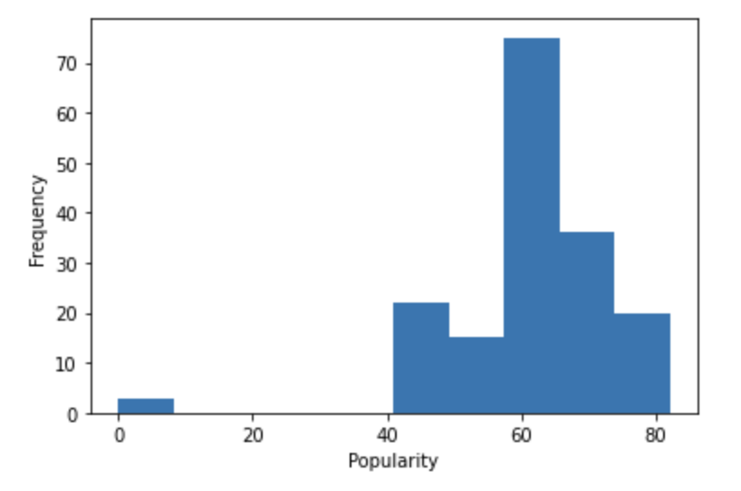
Generating/ Exploring Hypothesis
After looking over the dataset as a whole, we can start to manipulate it to look into our areas of interest.
By this point, we should have a solid understanding of the structure of our dataset. Now, you will think of 2-3 hypotheses or questions. These hypotheses or questions will be the basis of your project.
For example, how does X affect Y in this dataset? Can we predict Z using A? After formulating our hypothesis, creating DataFrames that take subsets of our main df, or grouping the data, is an excellent way to test our theories.
In this example, we'll examine differences in various categories of audio information based on album. First, let's group the data by album, and create different DataFrames for each albums. This will allow us to examine differences in Taylor Swift songs depending on the album a song was from.
One question we might like to answer is: "Is the median danceability in Taylor Swift songs different in each Album?"
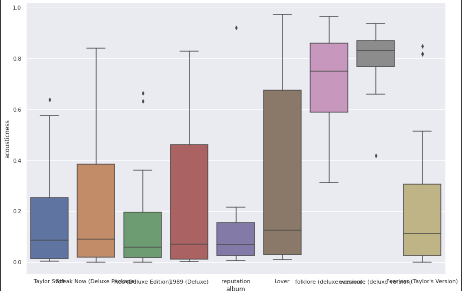
As we can see in the box plot below, the median danceability of her songs in Lover and Folklore are quite different. Creating plots and visualizations like this can help us to see patterns in our data that we might otherwise miss.
df.groupby('album').agg('mean').reset_index()| index | album | length | popularity | danceability | acousticness | energy | instrumentalness | liveness | loudness | speechiness | valence | tempo |
|---|---|---|---|---|---|---|---|---|---|---|---|---|
| 0 | 1989 (Deluxe) | 217139.3684 | 54.4211 | 0.6332 | 0.2446 | 0.6248 | 0.0007 | 0.2032 | -7.9241 | 0.1735 | 0.4542 | 127.0331 |
| 1 | Fearless (Taylor's Version) | 245865.0 | 65.5769 | 0.551 | 0.2141 | 0.6391 | 0.0 | 0.1624 | -6.1965 | 0.0379 | 0.4219 | 131.2372 |
| 2 | Lover | 206187.8333 | 72.1111 | 0.6582 | 0.3337 | 0.5452 | 0.0007 | 0.1152 | -8.0133 | 0.0991 | 0.4814 | 119.9727 |
| 3 | Red (Deluxe Edition) | 247294.3182 | 60.5 | 0.6334 | 0.1488 | 0.6008 | 0.0018 | 0.1191 | -7.38 | 0.0366 | 0.4681 | 110.2965 |
| 4 | Speak Now (Deluxe Package) | 275969.5 | 49.7273 | 0.559 | 0.2265 | 0.6594 | 0.0001 | 0.167 | -4.8069 | 0.0352 | 0.4297 | 132.8357 |
| 5 | Taylor Swift | 213971.1333 | 50.1333 | 0.5453 | 0.183 | 0.6643 | 0.0001 | 0.1608 | -4.7317 | 0.0327 | 0.4265 | 126.0538 |
| 6 | evermore (deluxe version) | 243816.2353 | 65.4706 | 0.5268 | 0.7941 | 0.4941 | 0.0206 | 0.1136 | -9.7816 | 0.0579 | 0.4335 | 120.7073 |
| 7 | folklore (deluxe version) | 236964.4706 | 62.6471 | 0.5419 | 0.7176 | 0.4158 | 0.0003 | 0.1105 | -10.3361 | 0.0395 | 0.3614 | 119.8844 |
| 8 | reputation | 223020.0 | 71.8667 | 0.6579 | 0.1385 | 0.5829 | 0.0 | 0.1522 | -7.6724 | 0.0951 | 0.2934 | 127.5401 |
evermore = df[ df.album == 'evermore (deluxe version)']
lover = df[ df.album == 'Lover']
print(lover.danceability.mean())
print(evermore.danceability.mean())
0.6582222222222223
0.5268235294117648
sns.set(rc={'figure.figsize':(5,5)})
sns.boxplot(x = 'album', y = 'danceability', data = df)
sns.set(rc={'figure.figsize':(5,5)})
sns.boxplot(x = 'album', y = 'acousticness', data = df)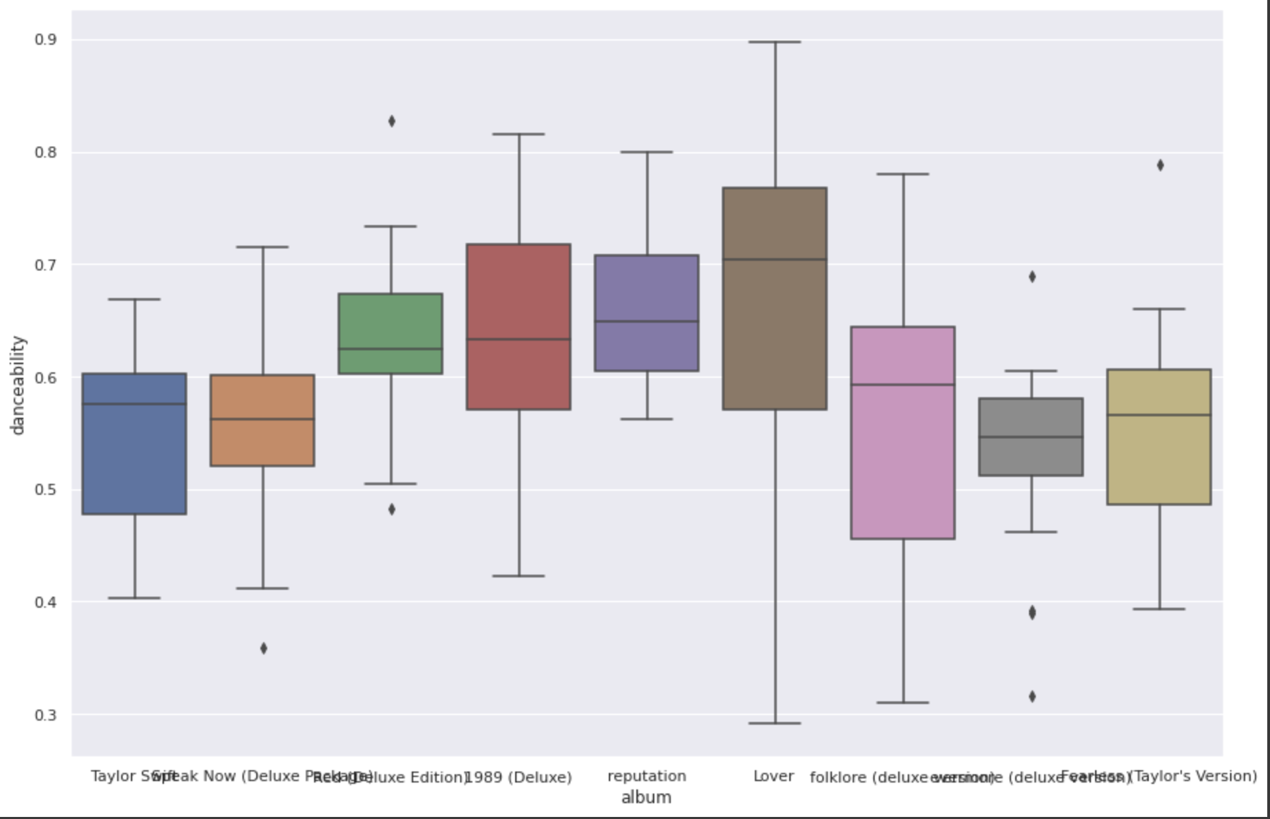
Statistical and Predictive Analysis
After diving further into your hypothesis, the time has come to perform our final analysis.
Now, we can take an observation we had (or something we want to predict) and create hypothesis tests, confidence intervals, linear regressions, or clustering models on our data. The steps above should help you identify variables that may be related or may affect another variable. Use these variables to conduct the above mentioned tests and prove, or disprove, your hypotheses.
This guide is only a suggestion on ways to get started. Your datasets will likely look quite different from the one we used here, but the principles we discussed can help you get started if you aren't sure how to begin! Good luck future data scientist.