Cross Validation in Python

In the field of Data Science, machine learning refers to a set of algorithms designed to predict outcomes more accurately. By analyzing large datasets, these algorithms can enhance their predictive capabilities and improve performance across various industries. Utilizing specific evaluation metrics, such as cross-validation, it is possible to assess the performance of a given model more effectively, which is a key part of the model selection process.

What is Cross Validation?

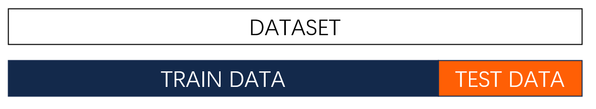
Cross Validation is an unsupervised machine learning algorithm that splits the dataset into a training dataset and a test dataset. The training dataset is fitted against the model, and the test dataset is used to simulate performance on new, unseen data. Thus, Cross Validation reserves a subset of the training observations from the fitting process to apply the learning model to those held-out observations. Some of the common Cross Validation forms are:

• Validation Set Approach
• Leave One Out
• K-Fold Cross Validation

Based on certain evaluation metrics, you can more effectively evaluate the model's performance (model assessment) and select the appropriate level of flexibility (model selection). Let’s explore these common Cross Validation forms in the following examples!

The Secrets of Cross Validation

A detailed explanation of machine learning algorithms can be found on the DISCOVERY website:

• Lecture: Linear Regression
• Lecture: Machine Learning Models in Python with sk-learn
• Lecture: Clustering

from sklearn.linear_model import LinearRegression

Step 2 - Create an Instance of the Model

The second step will always be to create a new instance of the model, which we will call model:

model = LinearRegression()

Since we have created a new instance of the model, we can use the diamond dataset to predict the price based on the size of the diamond. In this case, we are dealing with only one independent variable, which is the carat weight. So, we have a list containing a single element: carat. Then, we explicitly designate the dependent variable as price. This is because the model we're working with accommodates only one dependent variable, which is the target we aim to predict or analyze in our regression analysis.

Step 3 - Train the Model

import pandas as pd
df = pd.read_csv("https://waf.cs.illinois.edu/discovery/diamonds.csv")
model = model.fit( df[ ["carat"] ], df["price"] )

You've successfully fitted a model! Before you start celebrating and declare victory over the diamond datasets, you may wonder how well the model fits the data, whether the model is underfitting which occurs when a model is too simple to capture the underlying patterns or overfitting which occurs when a model so complex that it captures noise.

In this rest of this guide, we will explore how to use Cross Validation as a tool for evaluating datasets. In ideal cases, there will be a test dataset provided to the model in order to evaluate its performance according to certain metrics. However, such a test dataset may not be provided! That’s where Cross Validation (CV) comes into place.

The Validation Set

Before exploring different methods for Cross Validation, let's import some Python libraries that will assist us on our adventure exploring Cross Validation. Let's try it out!

# Import related libraries
import pandas as pd
from sklearn.linear_model import LinearRegression 
from sklearn.model_selection import train_test_split
from sklearn.model_selection import cross_val_score
from sklearn.model_selection import LeaveOneOut
from sklearn.metrics import mean_squared_error
import numpy as np

Since we already have all the libraries that we need, there is one more step before we can explore the power of Cross Validation. We need to split the data into features X and target y so that our Machine Learning algorithm can make predictions based on the new dataset.

# Prepare the data
X = df.drop(["price"], axis = 1)
y = df["price"]

Now, we are ready to utilize Cross Validation in our project! Let's split data by specifying the sizes of the train and test sets. Then, we will randomly divide the dataset into a training set and test set.

# Validation set approach
X_train, X_test, y_train, y_test = train_test_split(X, y, test_size=0.25, random_state=107)

Next, we have to train and validate the model by training the model on the training set and validating the trained model on the separate test set to assess its performance. In this example, our model is trained on the carat feature and the predictions are made on the same feature, which is a simple regression task where the goal is to predict the price of a diamond based on its carat size. Hence, we can use various machine learning algorithms, such as linear regression, decision trees, or neural networks, to make the predictions.

# Fit the model on the training data using only the "carat" feature
model.fit(X_train[["carat"]], y_train)
# Make predictions on the test set
pred = model.predict(X_test[["carat"]])

Based on the model that we have fitted, we can evaluate the model's performance on the test set. RMSE, known as the Root Mean Squared Error, is a widely used metric in machine learning for evaluating the performance of regression models. RMSE measures the average magnitude of the errors between the predicted values from a model and the actual values from the data. In addition, it also provides an indication of how accurately the model predicts the target variable. In this instance, the RMSE value of 1586.7504945497692 suggests that, on average, the model's predictions deviate from the actual values by approximately 1586.75 units. Thus, a lower RMSE indicates a more accurate model that can predict the target variable more closely to the actual values.

# Calculate the Root Mean Squared Error (RMSE)
RMSE = mean_squared_error(y_test, pred, squared=False)
# Print the RMSE
print("Root Mean Squared Error (RMSE):", RMSE)

Root Mean Squared Error (RMSE): 1586.7504945497692

As one can see, there are two potential drawbacks with this approach:

1. The estimate of the test error rate is highly variable due to the random split at the beginning; the observations that are included in training set and in test set play a crucial role on the outcome.
2. It overestimates the true error rate because statistical methods tend to perform worse when there are fewer observations for training.

The Magic of Leave-One-Out Cross Validation (LOOCV)

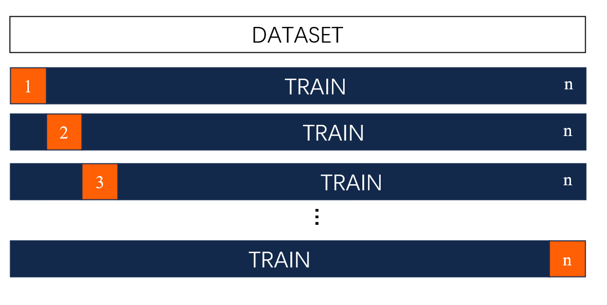
Leave-One-Out Cross Validation is a specific form of Cross Validation technique used to evaluate the performance of a machine learning model; it is most suitable for small datasets and provides an exhaustive and detailed evaluation of the model's performance.

Let's start Leave-One-Out Cross Validation by creating an instance using LeaveOneOut(). In LOOCV, each sample is used once as a test set while the remaining samples form the training set. This process repeats for each data point in the dataset, ensuring that every data point is used exactly once as part of the test set. Let's try it out!

# Perform Leave-One-Out Cross-Validation (LOOCV)
loo = LeaveOneOut()

We can use cross_val_score to evaluate a scoring metric across different splits of the dataset. By excluding the data point chosen for testing, we can use the trained model to predict the left-out data point.

# Use the "carat" feature for training in LOOCV
score = cross_val_score(model, X[["carat"]], y, cv=loo, scoring="neg_mean_squared_error")

Now, we can calculate the Root Mean Squared Error (RMSE) from the scores obtained in the Leave-One-Out Cross Validation (LOOCV) process. Since score contains negative values, we need to convert these negatives to positives, representing the Mean Squared Error (MSE) for each test set in the LOOCV process.

# Calculate RMSE for LOOCV
RMSE_LOOCV = np.sqrt(np.abs(score).mean())

# Print the RMSE for LOOCV
print("Root Mean Squared Error (LOOCV):", RMSE_LOOCV)

After carefully comparing the results between these validation set approaches, we can see that Leave-One-Out Cross Validation has the following advantages:

Reducing Bias

There is less bias or overestimation of the error rate because approximately twice as many observations are included in the training set.

Reducing Variance

Variance is reduced due to consistent results across multiple trials, as there are no random splits in Leave-One-Out Cross Validation, which avoids the risk of over-optimizing for a specific split.

However, the n models need to be fit to use Leave-One-Out Cross Validation, making it computationally expensive and time consuming to implement when n is extremely large.

The Mystery of K-Fold Cross Validation

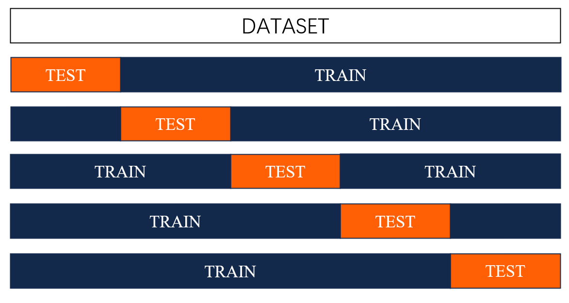
K-Fold Cross Validation is a powerful technique used to assess the predictivity of a machine learning model by dividing the data into k subsets and iteratively training the model k times, using a different subset as the test set and the remaining data as the training set. In addition, this approach helps in mitigating the variance in the model's performance evaluation. Moreover, the Leave-One-Out Cross Validation is a special case of K-fold Cross Validation where k = n. Let's delve into each part of K-Fold Validation:

1. Split Data: Randomly divide the dataset into k folds, using each fold as a validation set while the remaining data serves as the training set in each iteration. Let's try it out!

# Perform k-fold Cross-Validation (e.g., k=5)
k_fold_cv = 5

2. Train and Validate Model: For each iteration, train the model on the training set and validate it on the designated validation set.

# Use the "carat" feature for training in k-fold cross-validation
score_kfold = cross_val_score(model, X[["carat"]], y, cv=k_fold_cv, scoring="neg_mean_squared_error")

3. Evaluate Performance: Use certain metrics to evaluate the model's performance on the test set.

# Calculate RMSE for k-fold cross-validation
RMSE_kfold = np.sqrt(np.abs(score_kfold).mean())

# Print the RMSE for k-fold cross-validation
print("Root Mean Squared Error (k-fold CV):", RMSE_kfold)

Root Mean Squared Error (k-fold CV): 1938.0324820007454

Therefore, K-Fold Cross-Validation is a reliable method to minimize the chance of overfitting to a particular data split while being computationally efficient. When we are deciding on the number of folds k to use, there's a balance to be struck between bias and variance, which is a known as the bias-variance tradeoff. Conversely, Leave-One-Out Cross-Validation provides a nearly unbiased estimate of the model's error rate on unseen data but fitting models on similar dataset leads to highly correlated outputs and generates higher variance.

Unlock the Secrets of Cross Validation

You can read more about different types of Cross Validation from the Python documentation here.