Central Limit Theorem
The Central Limit Theorem, or the CLT, is one of the most important theorems in statistics! It says that:
Regardless of the distribution shape of the population, the sampling distribution of the sample mean becomes approximately normal as the sample size n increases (conservatively n ≥ 30).
In other words, if we repeatedly take independent random samples of size n from any population, then when n is large, the distribution of the sample means will approach a normal distribution.
This is very interesting and helps make our lives as data scientists easier! This means that doesn't matter if a distribution shape is left-skewed, right-skewed, uniform, binomial, or anything else - the distribution of the sample mean will always become normal as the sample size increases.
Because of the CLT, we can use the standard normal curve as an approximate histogram for the sample means. Also, we can use the standard normal curve to calculate areas just like we did previously with variables that were normally distributed.
Using the Standard Normal Curve and Random Variables
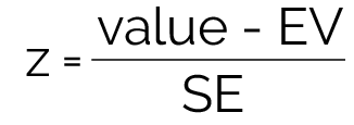
Remember, to use the Standard Normal Curve, we must convert our data to z-scores. It's important to point out that when dealing with random variables, our z-score formula changes slightly from the original z-score formula. Instead of average and SD, we are now dealing with average and SD of random variables. In other words, we need to use the expected value (EV) and standard error (SE) when we are dealing with random variables.
- Here's an example of how we can see the Central Limit Theorem in action. In this game, we win if we pick a queen from a deck of 52 cards -- try testing different values for "n":
2
A function drawForQueen that simulates of drawing n cards, counting the number of queens.
- We see that as
nincreases, our histogram looks more and more like the normal curve.
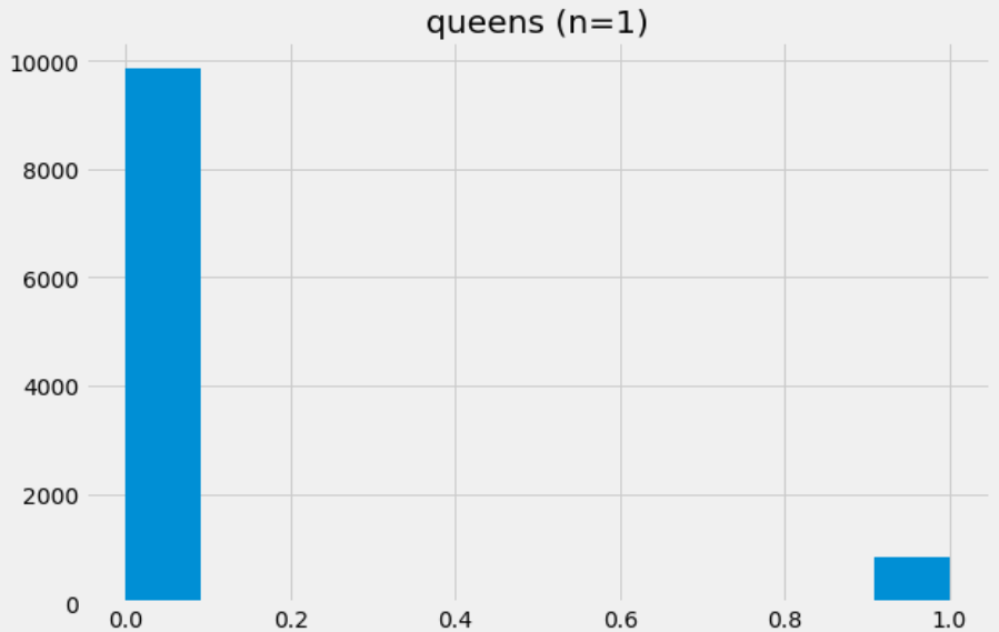
drawForQueen(1), creating a very lopsided distribution.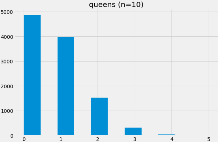
drawForQueen(10), creating a staircase-style distribution.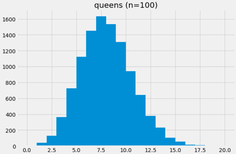
drawForQueen(100), creating a nearly normal distribution!
drawForQueen(1000), retaining and really showcasing the central limit theorem!