Grouping Data in Python

DataFrames are great tools for exploring data about individual observations, or rows, of data in a dataset. However, we often want to know about statistics on an entire category of data!

For example, the Illini Football Dataset contains all football games played by Illinois since 1892. When sorted by the Opponent you can see that we have played many teams more than once (in the full dataset, we've played some teams over 70 times!):

df = pd.read_csv("https://waf.cs.illinois.edu/discovery/football.csv")
df.sort_values("Opponent").head(20)

When we group data in a DataFrame, we are exploring data about all rows with similar data in one or more columns. Several questions we can ask about the Illini Football dataset includes:

• What was the average number of points scored by the Illini score against each opponent they played? Ex: How many points did the Illini score verses Purdue? ...verses Arizona? ...verses Nebraska? (We are grouping on different values in the Opponent column.)
• What is the standard deviation of points scored by the Illini in home games vs. away games? (The grouping on different values in the Location column, where vs. are home games and @ are away games.)

Using df.groupby to Create Groups

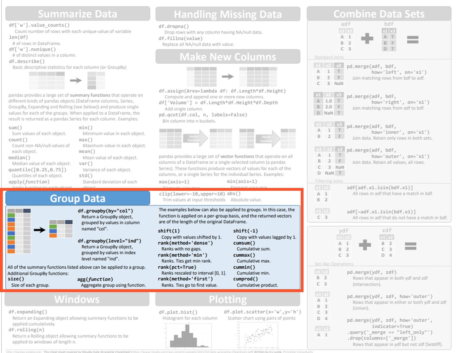
The pandas cheat sheet provides us an overview of the "Group Data" in Python:

Pandas Cheat Sheet, Page 2 with the "Group Data" section highlighted

"Group Data" section from Page 2 of the Pandas Cheat Sheet

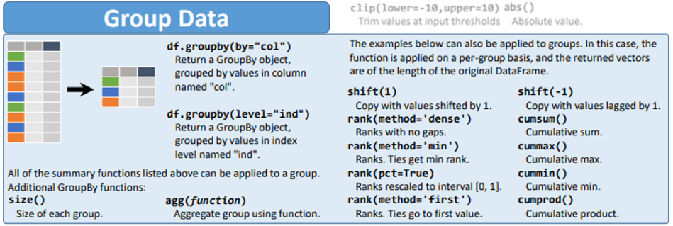
The syntax of groupby requires us to provide one or more columns to create groups of data. For example, if we group by only the Opponent column, the following command creates groups based on the unique values in the Opponent column:

df.groupby(by="Opponent")

Commonly, the by= argument name is excluded since it is not required for simple groups:

df.groupby("Opponent")   # Identical to by="Opponent" above

Internally pandas is creating many groups, where each group contains ALL rows that have the same value in Opponent. Looking at the twenty rows from the Illini Football Dataset again, I can highlight the different groups to show what pandas is doing:

Working with Group Data

Unfortunately, a group is complex and hard to visually represent so pandas will not provide any visual output when you create a group. Instead, we will either:

1. Use the group to explore summary statistics about each group (group.describe()), or
2. Aggregate all of the groups using a aggravation function (group.agg(...)).

We'll explore them both!

Viewing Summary Statistics of Group Data

When we create a group data in Python, we will commonly refer to the variable that contains the grouped data as group:

group = df.groupby("Opponent")
# group now contains our group data

On a group, group.describe() provides summary statistics of all numeric columns of data for each group. Using the same DataFrame with the Illini Football Data grouped by Opponent, we see the summary statistic of every group:

group = df.groupby("Opponent")
group.describe()

A few observations:

• The rows are now labeled with the Opponent. The rows will always be based on what we grouped our data by in the groupby command.
• The columns are all of the numeric categories in the dataset (Season, OpponentRank, IlliniScore, and OpponentScore).
• The sub-columns are various summary statistics (count is the number of total rows included in the group; mean is the average of the values of those rows; min is the minimum value, 50% is the median value, etc).

Aggregating Groups in Grouped Data

In many cases, we want to continue the analysis with a summary statistic of group data. On a group, group.agg(...) provides the ability to aggregate all rows within a group into a single value. There are hundreds of available functions, but a few are very common:

• df_count = group.agg("count") will count the number of rows in each group. This does not look at the data within the rows at all, it only counts how many rows are each group! For example, the Illini has played Akron only twice so the count is 2.

• df_mean = group.agg("mean") will find the mean (average) of each numeric column for each group. For example, the two Akron games the Illini scored 42 and 38. Therefore, the mean is 40.

• df_sum = group.agg("sum") will find the sum of each numeric column for each group. The sum of all the points the Illini scored against Akron is 80.

• Other strings that can be used include: "std" for each group's standard deviation, "median" for each group's median value, "var" for variance, and many more.

To make working with the DataFrame as simple as possible, we will ALWAYS use .reset_index() after .agg(...).

Example: Average Points Scored in Home vs. Away Games

I have always heard that a sports team has a "home team advantage", where they will preform better at home than away. Let's see if the Illini, on average, has scored more points at home or away?

Exploring the dataset, the Location column indicates if the game is played at home (vs.), at the opponent's stadium (@), or at a neutral site (ex: Memphis, TN):

Creating group data based rows that have the same value for Location, we use groupby:

group = df.groupby("Location")

Since we know we're interested in the average points, we can aggregate our group data together using "mean". The full Python code includes a groupby, an agg, and a reset_index:

group = df.groupby("Location")
df_mean = group.agg("mean").reset_index()
df_mean

There are quite a few neutral sites, so let's write a conditional on df_mean to display only the home and away games:

df_mean[ (df_mean.Location == "vs.") | (df_mean.Location == "@") ]

This DataFrame provides our answer! Specifically:

• When the Illini is playing games at home (when Location == "vs."), the Illini score an average of 21.1 points.
• When the Illini is playing games at the opponent's stadium (when Location == "@"), the Illini score an average of only 15.9 points.
• This is a very large difference (5.2 points) and suggests that the "home team advantage" may be a real thing!

Example Walk-Throughs with Worksheets

Video 1: Types of Variables

Video 2: Reading Histograms (Part 1)

Video 3: Reading Histograms (Part 2)

Practice Questions